1. Introduction

1.1. Urban mining and deep learning

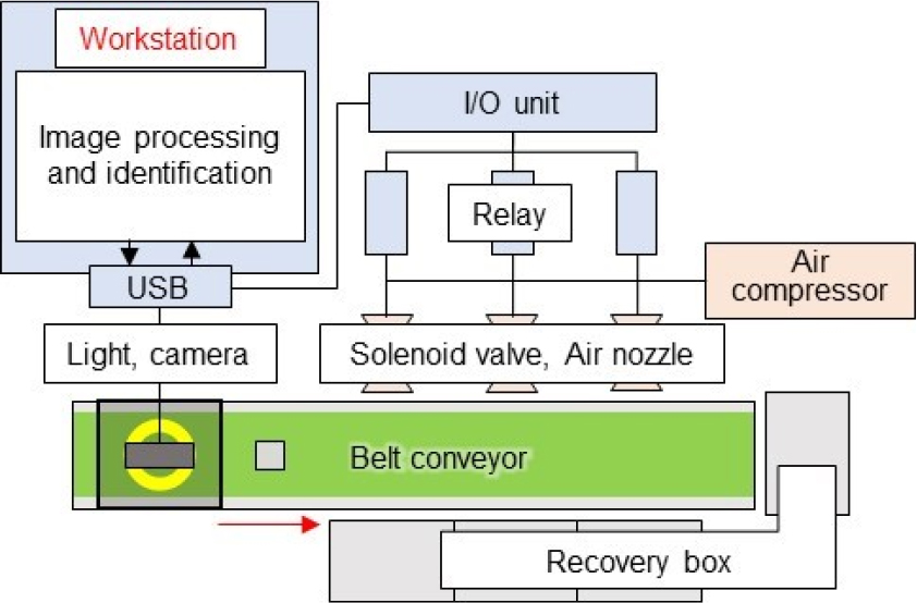
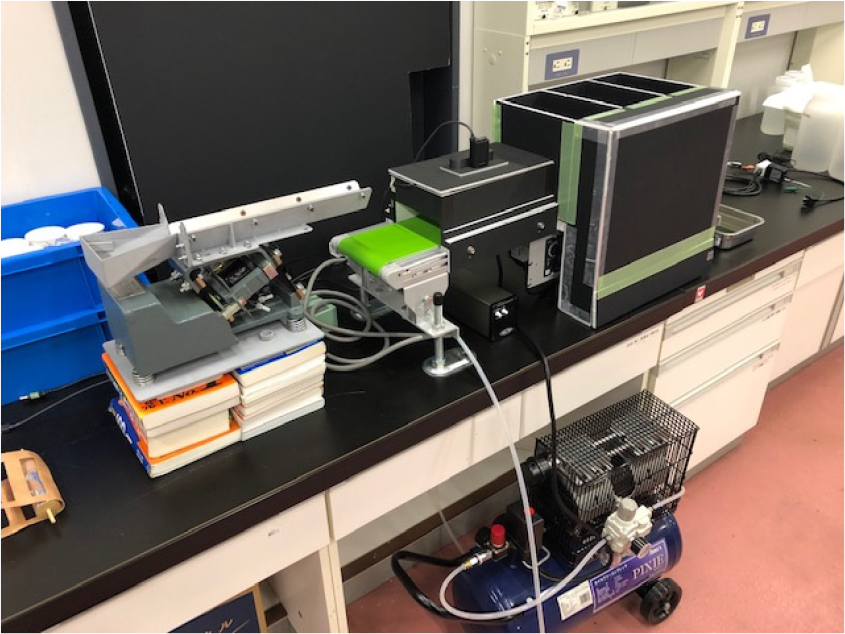
An urban mine is a stock of valuable metals in the discarded waste such as electronic equipment. As the underground resources are afraid to dry up someday, precious and rare metal prices have risen in recent years¹⁾. Therefore, taking out metal resources from urban mines, which are ground resources, is a part of recycling. The urban mines have more definite reserves and higher quality than the underground resources. Especially, waste mobile phones have a high content of rare metals. Therefore, recycling has been promoted. However, recycling methods for recovery have not been established to need the complex and expensive process for the composition of waste. Small home appliances such as mobile phones mostly consist of plastic and base metal. Electronic circuit boards and electronic components contain valuable metals including gold, but they are a little. Moreover, the content of the material and valuable metal is dependent on the type of electronic components. To recycle them efficiently, it is desirable to separate them in the intermediate process by the difference of valuable metals. Moreover, because even the same kind of components may physically vary and there are various physical sorting methods, it is difficult to conclude which method is optimal. Therefore, sorting technology that doesn’t depend on the physical properties of electronic components is required. In recent years, the field of artificial intelligence (AI) has particularly attracted attention as the “Fourth Industrial Revolution”. In machine learning, a statistical method for extracting the law from data, various algorithms for extracting the law and classifying have been proposed. In particular, the study on image identification has progressed significantly with the advent of deep learning. Today, the accuracy of the proposed image identification model exceeds the accuracy of humans²⁾. In this study, focusing on the point that image identification does not depend on the physical properties of electronic components, we manufactured a sorter with an electronic component identification model as shown in Fig. 1. Fig. 2 shows the photo of the sorter. This sorter can be separated the electronic components recovered by surface crushing the waste electronic circuit board into four groups. Parameters such as blow-out time of compressed air and belt speed were set. Therefore, the optimum condition was determined by evaluating the number of correct answers of image identification and the number of recoveries by blow-off by changing parameters.

Fig. 1.

Overview of sorter by image identification.

Fig. 2.

Photo of a sorter.

1.2. Image identification by deep learning

Image identification by deep learning uses a convolution neural network (CNN) that combines a feature extractor that includes convolution and pooling, and a classifier consisting of the fully connected network. Convolution takes out information in space such as straight lines and curves of the input image, and pooling manages out of position such as vertical and horizontal of the input image.

The fully connected network outputs a probability of prediction of classification from the input image.

Learning by CNN is to update the weight parameters on the network to get closer the predictions (outputs) from the network to the actual answer. Our image identification model can be created to learn with our image data set. In this study, it would be possible to reproduce the movement similar to hand sorting by the human brain and visual recognition by image identification and mechanical recovery method that didn’t depend on the physical properties of electronic components. CNN needs to create a model structure by setting the number of convolution layers and the parameters of the layers before learning. However, the advanced model structures provided by the library for deep learning, will not be necessary. It is called fine-tuning to relearn some or all of the weight parameters of models other than the output layer with our image data set. In this study, 140 kinds of electronic component images fine-tuned the GoogLeNet model (Xception), and an image identification model for them was created. The numbers of convolutions were depended on the accurate model. However, an accurate model was needed to increase the number of parameters and calculations. The GoogLeNet is an accurate identification technology to reduce the calculation amount while maintaining the deep convolution.

This model is used as an identification unit of the sorter shown in Fig. 1. TensorFlow, a library for deep learning made by Google, is free of charge, and we can easily implement CNN software by using this library. Using CUDA published by NVIDIA, deep learning calculations can be performed at high speed on NVIDIA GPUs. Therefore, if the sorting by image identification becomes more accurate and high-speed than the hand sorting, it is thought that the operation at high efficiency and low cost can be realized.

2. Experiment

2.1. The sorter of electronic component

The workstation which is the calculation unit in image identification used the GPU made by NVIDIA, and high-speed calculation was achieved by CUDA. The photography unit used a webcam that could be shot at 640 x 480 pixels and 60 FPS. LED ceiling lighting (Outer diameter 102 mm, inner diameter 52 mm) was pasted as a light source at the top of the box (Length 28 cm x Width 16 cm x Height 10 cm), it is surrounded by a white glossy paper on the inside, and in the center of the light, the webcam was put in from the outside of the box. In this way, it is possible to take a picture with a constant brightness to avoid the influence of the outside brightness. The belt conveyor had a yellow-green belt (Length 100 cm, belt width 14 cm) to recognize the background difference while photographing. To recover the electronic components that passed through the photography unit by blowing off with compressed air, the recovery unit (three solenoid valves and three air nozzles) was installed at 13 cm intervals on the side of the belt conveyor. The recovery box was placed on the opposite side of the solenoid valves and air nozzles. To prevent the scattering of electronic components by blowing off, the recovery box from the air nozzle was enclosed with a plate other than the top. Fig. 3 shows the process to get an electronic component image.

Fig. 3.

The process to get an electronic component image.

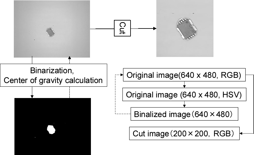
First, the center of gravity was got by calculating from the binarized object portion by the background difference of photographed image. Next, the original image before the background difference was got when the center of gravity passes through the center (320 pixels in horizontal). Finally, a square of 100 pixels from the center of gravity was cut, and an image of 200 x 200 pixels (3.5 cm x 3.5 cm in real size) was output. The actual size of the sample was from 5 mm for a resistor to 30 mm for a connecter. Image processing and signal of the opening and closing for solenoid valves, and the learning program were written by Python. The camera input was programmed by wrapping the C++ library in Python to achieve 60 FPS.

2.2. Image data set of electronic components

Electronic components were sorted by type. If the shape was different in the viewpoint direction, it was a different class on the image data set. The electronic component image was classified into the following four groups by the difference of refinement process in the recycling process. The photos of samples are shown in Fig. 4. The size of most samples was several mm. The aspect ratio was almost 1 to 2. Some ICs and connectors had large aspect ratios such as 5 to 10.

Fig. 4.

The photos of samples for 4 groups.

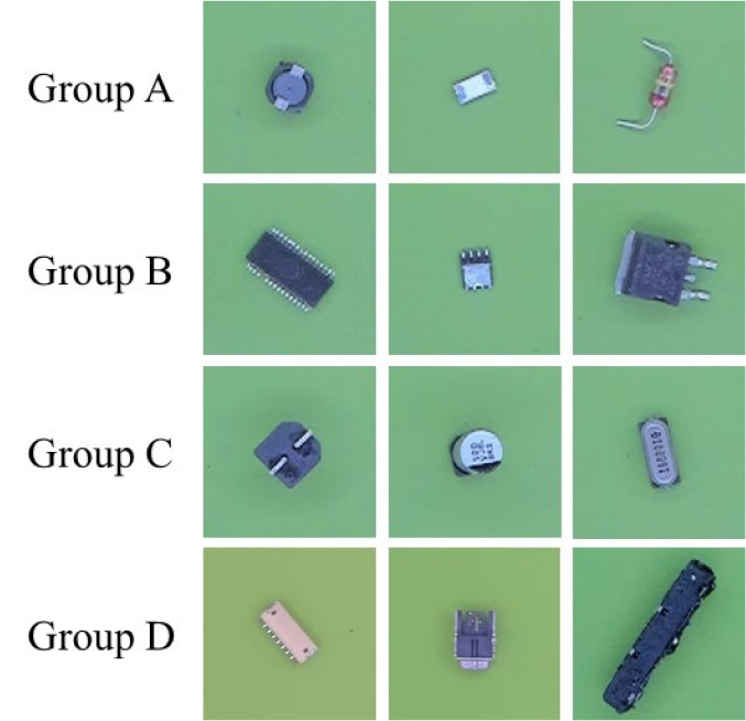
(Group A) A group that doesn’t contain gold or aluminum. 60 types of the example including coil, resistor, and diode.

(Group B) A group that contains gold but is molded by epoxy resins, which require combustion processing such as ICs and transistors. 61 types of the example including IC and transistor.

(Group C) A group that contains aluminum, which is an interfering substance of reaction in the wet processing. 13 types of the example including condenser and quartz oscillator.

(Group D) A group such as connectors that is gold- plated. 6 types of the example including connector.

To collect images of electronic components, electronic components were supplied by hand so that they didn’t overlap on the belt conveyor that was flowing at 6 cm/s. 25 photos were taken in each type and a total of 140 kinds (3,500 images) output. These images were rotated at an angle of 90°, 180°, 270°, and three images were generated per image. These image data were teaching data (data set) for learning. Of these, a total of 10,500 images that are inflated by rotation were training data, and 3,500 original images were validation data (training: validation = 3: 1). GoogLeNet's Xception model was used for fine-tuning because of its accuracy. The classification method was supervised learning.

2.3. Change the setting value of the sorter

Belt speed, blowing time of the compressed air, and pressure of compressed air can be changed in the sorter. 25 electronic component samples (100 total) of each group were prepared as test samples. First, the belt speed was changed in the range of 6 to 21 cm/s, and the number of correct answers in each group for image identification was compared. Next, the blowing time of compressed air was changed in the range of 0.02 to 1.0 s for each belt speed, and the number of recoveries by spout out from the belt off was compared. From these results, the setting value of the sorting experiment was determined. In addition, the program was improved based on the behavior of recovery samples and the characteristics of the samples that failed to recover them. Furthermore, it was compared the number of recoveries by pressure change of compressed air. The optimum condition in the sorting was determined. In the sorting experiment, four groups of samples were sorted under the optimal condition.

3. Results and discussion

3.1. Fine-tuning with Xception models

To sort electronic components by image identification, it is necessary to identify the type of electronic component with high accuracy. Fig. 5 shows the learning curve in teaching data including 140 kinds of electronic components.

Fig. 5.

Learning curve in 140 electronic component images.

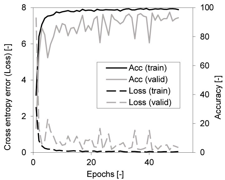
In this learning, when the epoch number (number of learning) was 41, the validation loss (cross-entropy error) was minimized. The validation accuracy at that time was 96.3%. Moreover, when classified by group, the group validation accuracy was 98.7% because the wrong answer between each group became correct in the same group.

3.2. Finding and implementing the optimal conditions in the sorter

When image identification can be processed at high speed, it is necessary to speed up to supply waste electronic components to sort a large amount of them. In this experiment, it is hand-supplied, but using feeders, it can be supplied intermittently with a large amount of waste electronic components. However, if the belt speed is slow with the feeder, electronic components are piled, and it becomes difficult to take photos and identify correctly. Fig. 6 shows the relationship between the belt speed and the number of groups correct answers for image identification of the test sample. It shows the biggest number of group correct answers when the belt speed was 6 cm/s at which the teaching data is taken. This result was the same level of image validation accuracy. It shows the least number at 21 cm/s, it is the maximum speed in the range. The optimal belt speed was determined at 18 cm/s when the number was almost the same from 9 to 18 cm/s in Fig. 6.

Fig. 6.

The relationship between the belt speed and the number of group correct answers of image identification of test sample.

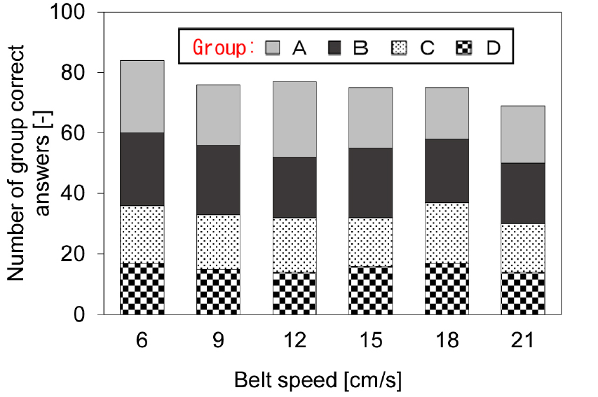
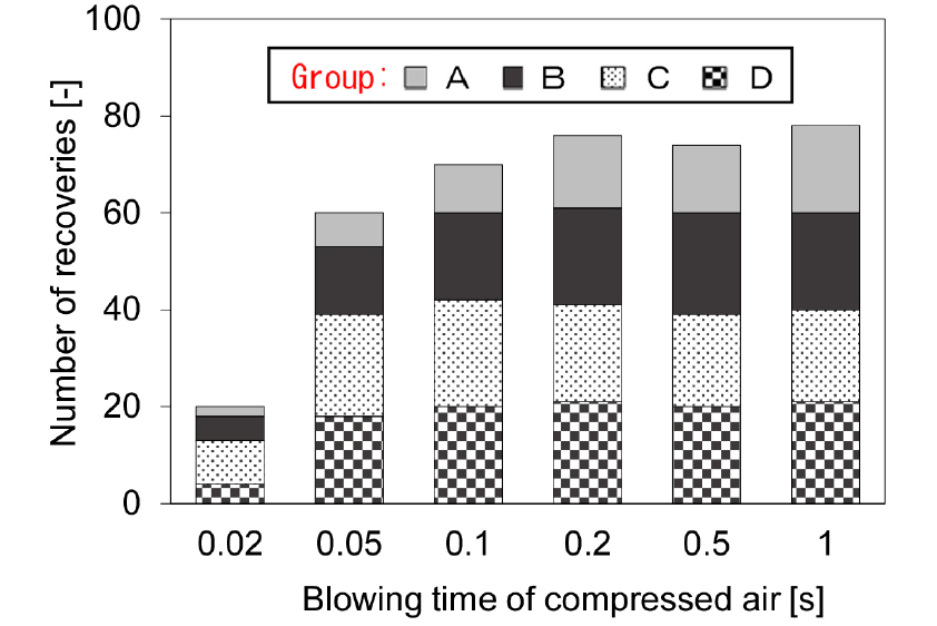
Fig. 7 shows the relationship between blowing time by compressed air and the number of recoveries in the blow at a belt speed of 18 cm/s. In this experiment, the test sample is blown by one air nozzle (air pressure: 0.2 MPa). When the blowing time was longer, the number of recoveries was bigger. The number of recoveries exceeded 75 at 0.2 s, and it was almost the same until 1.0 s. The electronic components must be supplied every 18 cm. When taking a picture of electronic components, the interval time was provided. When the component of Group A and Group B are supplied continuously, both of them were recovered in the same recovery unit for a longer blowing time than the interval time. When considered to prevent it, the following equation holds.

In this equation, ti_min is the minimum interval time when taking a picture, w_pic is the width of the actual size to get the image (200×200 pixels), v_belt is belt speed, and t_air is the blowing time of compressed air. In this experiment, because the w_pic was 3.5 cm and the v_belt was 18 cm/s, ti_min was 0.19 s and t_air was 0.2 s. However, because it was not possible to supply at a faster than 0.2 s in the hand supply, the blowing time was determined as 0.2 s.

Fig. 7.

The relationship between blowing time by compressed air and the number of recoveries in the blow at a belt speed of 18 cm/s.

It was decided to recover the sample of Group A at the front bottom of the belt conveyor rather than the recovery by blowing because the number of recoveries in Group A was smaller than in the other groups. In addition, the air pressure was changed from 0.2 to 0.4 MPa to increase the number of recoveries. The blowing point was not adjusted to the center of the sample when the belt speed was increased. The program was improved to blow the electronic components at a little in front of the center. Fig. 8 shows the number of recoveries after changing air pressure and the program improvement at blowing time: 0.2 s and at the belt speed: 18 cm/s. The changes in air pressure and the program improvements brought to increase in the number of recoveries. As the result, the optimal condition was determined that the belt speed was 18 cm/s, the blowing time was 0.2 s, and the air pressure was 0.4 MPa. The sorting experiment was conducted using the improved program under the optimal condition.

Fig. 8.

The number of recoveries after changing air pressure and the program improvement at blowing time: 0.2 s and at the belt speed: 18 cm/s.

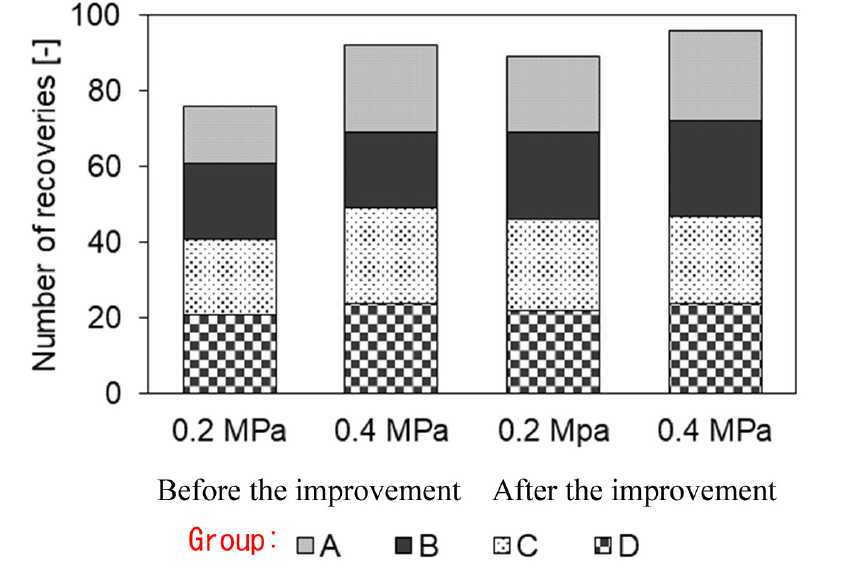
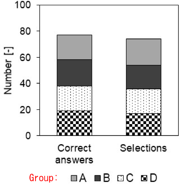
Fig. 9 shows the number of group correct answers and the selection number by image identification under optimal conditions. In this experiment, the selection number means the sum of the sample number that is recovered as the correct group in the recovery box installed in each group. Group correct answers were 77, and 74 samples were selected in the correct box. For the 100 samples, 4 samples were selected in the wrong box by mistake. One sample of Group A was recognized to another group, but because it was not selected by blowing correctly, there were three differences between the number of group correct answers and the selection number. It is thought that it is most important to improve the correct answer rate of image identification to increase the number of selections.

Fig. 9.

The number of the group correct answers and selection by image identification under optimal conditions.

4. Conclusion

In this study, an electronic component sorter was developed by image identification based on deep learning. As changing the conditions related to sorting by comparing and considering the results, the optimal conditions for the experiment and the program improvement were performed and the correct selection number was increased. The number of selections was 70%. It was not still a sufficient level. However, we believe that the possibility of AI in the recycling field was shown on a different approach using image identification by deep learning rather than the traditional physical sorting method. Currently, researches in the AI field are actively carried out, and as image identification is necessary for self- driving technology, it is expected that further progress will be made in the future. The accuracy rate of image identification was the most important for the AI sorting. We think it is necessary to continue researching the part of image identification for the future recycling field.